

Conjointly surveyed 3,970 voters in Australia to compare online survey results and actual 2025 Australian election outcomes, revealing the value of survey research for political polling and opportunities to better align survey data with real-world behaviour.
Online surveys can be a powerful tool for estimating real-world behaviour, but the quality of that estimate depends heavily on how the survey is designed and analysed. Decisions for sampling, question wording, and analysis can make a meaningful difference in how closely the results track reality. To investigate these dynamics, Conjointly launched a survey alongside the 2025 Australian federal election to compare survey results to real-life election outcomes. This overview describes details of the study, dives into key findings, and provides takeaways for launching surveys that accurately capture real-life respondent behaviour.
Pitting Survey Results Against a Real Election
Conjointly surveyed 3,970 Australian voters online during the 2025 national election, held May 3, 2025. The survey was open to any voter, regardless of whether they’d already voted (in person, by mail, or early) or hadn’t yet cast a ballot. Data collection ran for five days: from April 30 (three days before election day) through May 4 (one day after polls closed). Of the respondents, 51% had already voted at the time they completed the survey, while 49% completed it before submitting their ballot.
We gathered a representative sample using soft quotas to align our respondent pool with the Australian population of voters. Distribution across states and territories matched census data [1] within one percentage point, and responses were generally well-distributed across gender and age groups with a slight underrepresentation among older citizens.
Sample & Population Distribution by Age
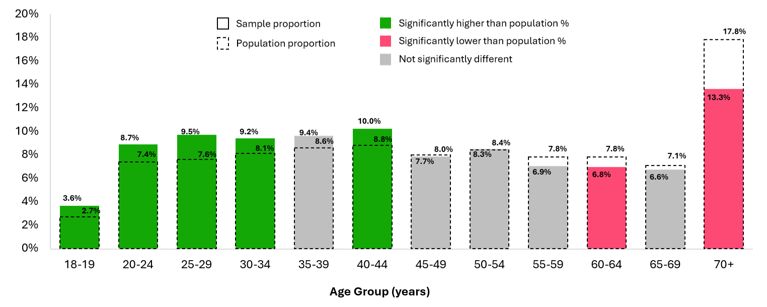
Figure 1 sample proportion data from 3,970 survey respondents, and population proportion data sourced from IBISWorld 2026: Population aged 18 and older in Australia [1].
The survey closely mirrored how the polls function in Australia, with respondents ranking the full list of candidates in their electorate for the House of Representatives. Respondents were also asked to share their vote “above the line” for the Senate, meaning they ranked each party available across Senate candidates in their territory or state.
For our analysis, we carried out three separate calculations from the survey data and compared them to the results reported by the Australian Electoral Commission for the 2025 election [3][6]. These comparisons gave us three metrics to determine the effectiveness of the survey:
House hit rate - We used a ranked choice voting process to determine the House winners in each electorate according to the survey. Using the ranked choice voting calculation, we measured hit rate — the percentage of electorates where the survey’s projected winner matched the actual winning candidate.
House two-party preference (2PP) - We calculated the margin between the percentage of respondents who prefer Liberal candidates and the percentage of respondents who prefer Labor candidates (the two largest political parties in Australia). Party preferences were determined by whether each respondent ranked the Labor House candidate in their electorate higher than the Liberal one, or vice versa. We then compared these margins to the actual results to evaluate how large the differences were.
Senate first preference hit rate - First party preference in the Senate is defined for each territory and state as the party with the highest percentage of respondents ranking that party at the top of their list [6]. We determined the first preference hit rate from our survey to be the percent of territories where the first preference party from our survey matched correctly with the actual results.
How Close Did the Survey Get?
Across 150 electorates, the survey correctly identified the House winner in 95 seats, a hit rate of 63%. To benchmark the effectiveness of our survey results, we compared our key metrics to those measured by traditional political polling companies. Our 63% hit rate was slightly lower than the accuracy of industry-leading polls like YouGov, which correctly predicted 112 winners for a hit rate of 75% [2].
Electorates Where Survey Winners Match Actual Winners
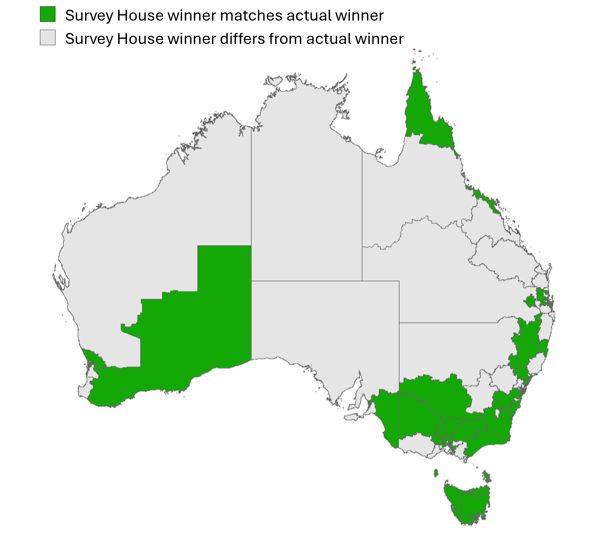
Figure 2 survey House winners calculated from 3,970 survey respondents, and actual House winners sourced from Australian Electoral Commission: 2025 federal election: House of Representatives results [3].
While the survey did not perform as well as traditional political polls on hit rate, it did a better job estimating the two-party preference metric. The national two-party preference metric in the survey deviated from the actual by 2.5%, compared to a 10%+ deviation for most polls according to Guardian [4]. Guardian’s article summarising two-party preference predictions from nine different polling organisations shows that the traditional political polls like Newspoll and Resolve predicted only a 2%-6% split between Labor and Liberal preferences, while our survey was much closer to the actual results.
National Two-Party Preference Results
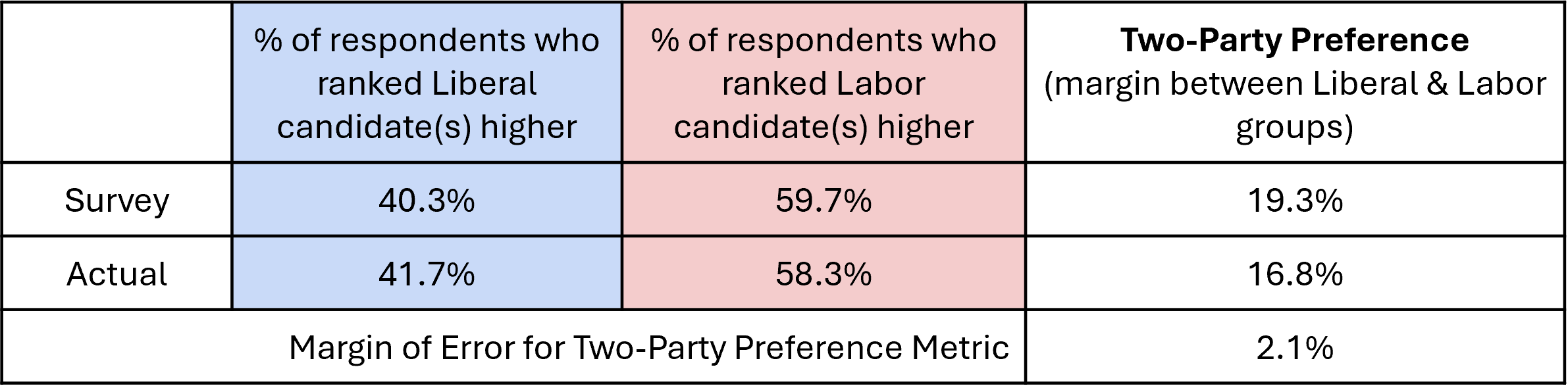
Table 1 survey 2PP results calculated from 3,970 survey respondents, and actual House two-party preference statistics sourced from Australian Electoral Commission: 2025 federal election: House of Representatives results [3].
This revealed an interesting dynamic: how could the two-party preference have been so close when the hit rate was comparatively low? The answer lies in the complexity of these metrics. While the hit rate was based on ranked choice voting, the two-party preference was a simple percentage statistic. The accuracy of the ranked choice results depended on how accurately people ranked every candidate on the list in front of them, while two-party preference only depended on whether they ranked the Liberal candidate over the Labor one.
To investigate further, we carried out bias detection to evaluate all potential sources of error in our sample, questionnaire, and analysis, and it was clear that the length of the candidate lists was impacting the results. Pasek & Krosnick’s research from 2010 shows that ranking lists longer than seven items are cognitively challenging for survey participants [5], and they often rank the top few options accurately while arbitrarily sorting the rest just to get past the question. In our study, the hit rate among electorates with less than seven House candidates (half our total 150 electorates) was 71%, compared to only 56% for electorates with seven or more House candidates. This indicated that even though the survey was designed to mirror real-life polling circumstances, respondents may not have fully reviewed and ranked all of their choices as they would on their actual ballot, focusing instead on their top one or two. Considering the ranked choice voting calculation for hit rate depended on respondents ranking all candidates as they would have during the election, the lower accuracy of House results from our survey could have been attributed to the larger cognitive capacity required to rank a full list.
The Senate first preference results affirmed the hypothesis that respondents focused on ranking their top options accurately rather than giving attention to entire lists. In our survey, the Senate first preference party matched the actual first preference party in 75% of the territories and states (6 out of 8). Furthermore, the Senate first preference hit rate among territories and states with less than 15 parties to rank was 67% (2 out of 3) compared to 80% for electorates with 15+ parties (4 out of 5), showing that people had the cognitive capacity to make sure their #1 was right even when presented with longer lists.
For this reason, one of the biggest takeaways from the analysis was to carefully consider key metrics and if they can be fully captured in an online survey. In this case, the length of the lists respondents had to rank online affected their cognitive capacity to share their votes, making the first preference or two-party preference metrics more effective than the hit rate. Clearly defining metrics and thoughtfully designing the survey to ensure the questions that support them are relevant is critical for accurately gauging real-life behaviour.
Methods to Transform the Data to Get Even Closer
There were three main approaches we used to shift the survey results closer to the actual election outcomes: weighting, small area estimation, and regression modelling.
Weighting
Using national demographics [1], we developed weighting schemes for the election dataset based on gender, age, territories and states, and nested subgroups. Note that we did not include income or race in the survey. The key metrics show that, in general, weighting negatively impacted hit rate, improved two-party preference accuracy, and had little effect on Senate first preference hit rate.
Evaluation of Different Weighting Schemes Across Key Metrics
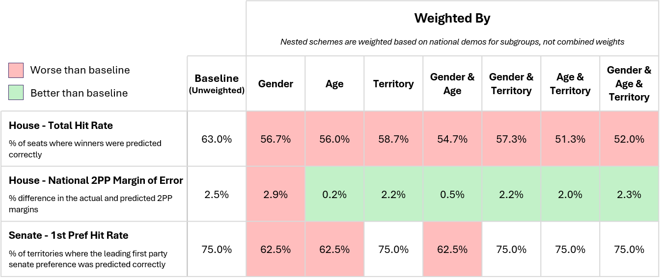
Table 2 survey metrics calculated from 3,970 survey respondents, and actual House and Senate results sourced from Australian Electoral Commission: 2025 federal election: House of Representatives results [3] and Senate state and territory results [6].
Weighting by age was the most effective approach to improve the two-party preference margin from the survey to within 0.016% of the actual margin. This aligns with our knowledge that older voters were underrepresented in our sample, so accounting for this via weighting gave them proper representation. Interestingly, nested weighting schemes were not more impactful than the simple weighting schemes.
But why did the House hit rate worsen for each of our weighting schemes? Again, consider how the metric is calculated. When weights are applied in the ranked choice voting process, which occurs within a smaller sample size at the electorate level, the weights given to each respondent at the national level may no longer be representative. In comparison, the two-party preference metric is a simple proportion calculated on the national level, so the weights are more likely to improve representation of certain groups rather than distort it. While weighting helps to smooth overall results, as you drill down into specific regions with smaller sample sizes, it may not be the most appropriate tactic. This is why we also applied small area estimation.
Small Area Estimation
Small area estimation (SAE) is a statistical modelling methodology designed to provide reliable estimates of population statistics in small geographical regions [7]. Originally used in epidemiology for estimating disease prevalence as well as poverty rates and healthcare access [8], SAE was very helpful in this context to extrapolate from the small samples in the less populated electorates. Since the SAE model we leveraged [9] required individual counts as inputs rather than ranked choice data, we decided to conduct the SAE analysis on the two-party preference metric in each electorate. In addition to the counts from the survey, the model also used external data for expected counts, which we pulled from the 2022 federal election [10], and a neighbourhood matrix [11] to “borrow” information from neighbouring regions to better understand the findings in regions with smaller sample sizes. We were lucky enough to have external data to strengthen the model, but this is not always possible, especially with new product and consumer behaviour research. Alternative SAE approaches can be applied when no external data is available [12].
Comparing results by electorate before and after the SAE model was applied, 78% of electorates saw an improvement in the difference between the survey and actual two-party preference margins. Additionally, across all seats, the average improvement in the difference between the estimated percentage of Liberal-leaning voters and the actual percentage of Liberal leaning voters was 5.8%. This average improvement was even greater among the 50 electorates with the smallest populations, 7.3%. When working with specific regional markets or hard-to-reach profiles, SAE can be a powerful tool for accurately estimating real-world behaviour.
Regression Modelling
Another helpful analysis technique we applied was regression modelling, specifically binary hierarchical logistic regression. In addition to House candidate and Senate party rankings, the survey also asked respondents to indicate issues that were important to them (economy, healthcare, immigration, etc.) as well as their satisfaction with the current Labor government’s performance on a scale of 1 to 5. We were curious if we could leverage that additional information to better estimate a respondent’s voting behaviour, but unlike the other analyses, we did not have real-world election outcomes with data about values to compare our survey results to. Instead, we split 60% of respondents into a training dataset to build the model and 40% into a test dataset to apply the model.
For this analysis, we used the two-party preference metric as our dependent variable because it was a value we could determine on an individual respondent level (1 if they preferred Liberal candidates, 0 if they preferred Labor candidates). We used demographics, important issues, and government satisfaction ratings as our independent variables, and the hierarchical regression approach allowed us to control for demographics to see if party preference could be predicted using just demographics or if values significantly contributed to respondents’ votes.
Overall, our model was moderately effective. We were able to apply it to the test dataset and correctly categorise respondents’ party preference 75% of the time (1,192 out of 1,584 test respondents) based only on their values and government satisfaction ratings. However, this accuracy lessened as we zoomed in at an electorate level. 18 seats based on model results had a significantly different two-party preference than the real-world results, compared to only 10 for the baseline survey output. These results indicated that binary logistic regression may have been useful for transforming our survey data, but it was likely not the best way. While the model was right 75% of the time, the Tjur’s R-squared was only 0.38. Tjur’s R-squared ranges between 0 and 1 and indicates how well a binary logistic regression model separates the two groups, in our case, those who prefer Liberal candidates and those who prefer Labor candidates. A value of 0.38 was not bad, but it was not enough for us to feel confident in leveraging this binary logistic regression model to improve the accuracy of our results.
The good news was that the important issues and government satisfaction were significant predictors of party preference while controlling for demographics (based on ANOVA results for the binary hierarchical logistic regression with a p-value of 2.2e-16). The output of the binary logistic regression highlighted the drivers for a greater likelihood of preferring the Liberal party.
Full Model Regression Output for Value Predictors
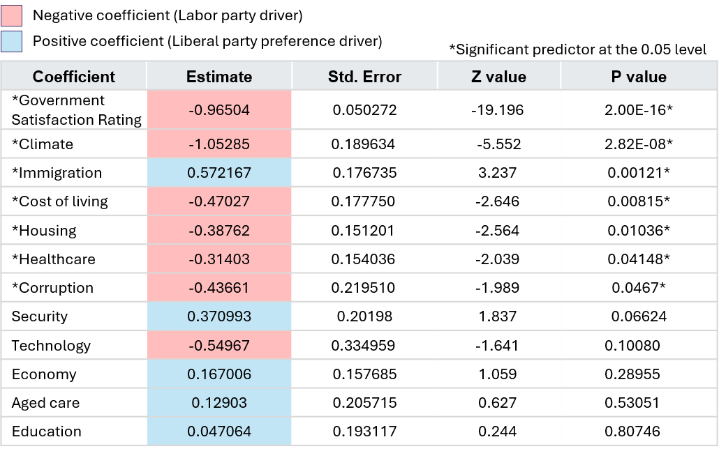
Table 3 regression results based on 2,386 responses in our randomly assigned training dataset.
These significant predictors align with party values. Issues like the economy, security, and immigration have positive coefficients that drive preference for the Liberal party, while healthcare, climate change and the environment, housing affordability, cost of living, and corruption have negative coefficients favoring Labor. Additionally, a higher satisfaction rating is associated with a lower likelihood of having a Liberal preference (negative coefficient), which makes sense considering Australia is currently run by a Labor government.
Despite the imprecision of our current regression model, this analysis highlights the opportunity to incorporate personal values into polling processes. As the political climate becomes more polarised, especially around climate change [13], understanding the nuances within parties will be informative.
Bridging the Gap Between Surveys and Reality
Predicting real-world behaviour through online surveys is a nuanced process. As the 2025 Australian federal election case study demonstrates, an online survey can be a highly accurate tool, sometimes even outperforming traditional political polls, but its success relies heavily on careful survey design, metric selection, and post-collection analysis. By comparing our survey data directly to real election outcomes, we uncovered several critical lessons for researchers looking to capture authentic behavioural intent:
- Thoughtfully determine how to best capture your key metrics: Complex survey tasks can degrade data quality. The drop in accuracy for electorates with seven or more candidates suggests that respondents may not fully engage with exhaustive ranked-choice lists online. When possible, consider more robust, respondent-friendly ranking methodologies like MaxDiff, or prioritise simpler, high-level metrics (like the 2PP), which yielded greater accuracy with only a 2.5% deviation from the actual.
- Apply weighting strategically: Demographic weighting, particularly by age, was most effective at correcting national-level metrics. However, applying those same national weights to smaller, electorate-level samples actually worsened the hit rate. Always consider the dynamics of the metrics you are analysing before applying broad weights.
- Leverage small area estimation for targeted accuracy: When you need to drill down into specific regional markets or hard-to-reach profiles, standard weighting falls short. Using SAE reduced the difference between survey and actual results in over 86% of electorates by borrowing contextual data, making it an essential tool for localised predictions.
- Look beyond standard demographics: While demographics are foundational, our regression analysis proved that personal values and satisfaction are significant predictors of behaviour in their own right. Incorporating these psychographic variables can provide much deeper context and predictive power than demographics alone.
Ultimately, online surveys are not a direct mirror of reality, but rather a powerful lens. By understanding the limitations of respondent fatigue and applying the right statistical models to the right sample sizes, researchers can confidently bridge the gap between survey intent and real-world action.
References
[1] Population aged 18 and older in Australia - Data and analysis (1971–2033), IBISWorld, 2026.
[2] YouGov was the most accurate pollster of the 2025 Australian federal election, Patrick English, YouGov, 13 May 2025.
[3] 2025 federal election: House of Representatives results, Australian Electoral Commission, 10 June 2025.
[4] The polls were off in Australia’s election – but it’s the uniformity that has experts really asking questions, Josh Nicholas & Tory Shepherd, The Guardian, 7 May 2025.
[5] Optimizing Survey Questionnaire Design in Political Science, Josh Pasek & Jon A. Krosnick, The Oxford Handbook of American Elections and Political Behavior, 2 May 2010.
[6] 2025 federal election: Senate state and territory results, Australian Electoral Commission, 30 May 2025.
[7] Bayesian statistics for small area estimation, Gómez-Rubio et al., Imperial College London, National Centre for Research Methods, 2010.
[8] Historical overview of small area estimation in the 50th birthday of the IASS, Isabel Molina & J. N. K. Rao, The Survey Statistician, July 2023.
[9] CARBayes: An R package for Bayesian spatial modeling with conditional autoregressive priors, Duncan Lee, Journal of Statistical Software, 20 November 2023.
[10] 2022 federal election: House of Representatives downloads, Australian Electoral Commission, 1 July 2022.
[11] Federal electoral boundary GIS data for free download, Australian Electoral Commission, 4 March 2025.
[12] Methods for Sampling and Inference with Non-Probability Samples, Lenau et al., InGRID-2: Integrating Research Infrastructure for European Expertise on Inclusive Growth from Data to Policy, September 2021.
[13] From ‘Lost Decade’ to incomplete ‘transformation’: Australian climate policy via ideas, interests, and institutions, Hopkinson et al., Australian Journal of Political Science, 4 October 2025.